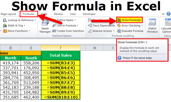
Getting The Excel If Formula To Work

By pressing ctrl+shift+center, this will compute and also return value from multiple ranges, as opposed to simply individual cells contributed to or multiplied by one another. Determining the sum, product, or quotient of specific cells is easy-- just use the =AMOUNT formula and enter the cells, worths, or array of cells you wish to perform that math on.

If you're seeking to discover total sales earnings from a number of marketed systems, for instance, the selection formula in Excel is ideal for you. Right here's how you 'd do it: To start utilizing the range formula, type "=SUM," as well as in parentheses, get in the first of two (or 3, or 4) ranges of cells you would love to increase with each other.

This means multiplication. Following this asterisk, enter your 2nd variety of cells. You'll be increasing this second series of cells by the initial. Your progress in this formula should now look like this: =AMOUNT(C 2: C 5 * D 2:D 5) Ready to push Enter? Not so fast ... Due to the fact that this formula is so complicated, Excel books a different key-board command for selections.

This will certainly acknowledge your formula as an array, covering your formula in brace personalities and successfully returning your item of both varieties combined. In profits estimations, this can minimize your effort and time significantly. See the final formula in the screenshot over. The COUNT formula in Excel is represented =COUNT(Start Cell: End Cell).

As an example, if there are eight cells with gotten in values between A 1 as well as A 10, =MATTER(A 1: A 10) will return a value of 8. The MATTER formula in Excel is specifically useful for huge spreadsheets, where you want to see the amount of cells include actual entries. Don't be misleaded: This formula will not do any mathematics on the worths of the cells themselves.

Interview Questions Can Be Fun For Everyone

Making use of the formula in bold above, you can conveniently run a count of current cells in your spread sheet. The outcome will look a something similar to this: To do the typical formula in Excel, enter the values, cells, or series of cells of which you're calculating the standard in the style, =AVERAGE(number 1, number 2, etc.) or =STANDARD(Start Worth: End Worth).

Finding the standard of a variety of cells in Excel keeps you from needing to locate individual sums and after that executing a separate department formula on your overall. Making use of =AVERAGE as your initial message entrance, you can allow Excel do all the work for you. For recommendation, the average of a group of numbers amounts to the sum of those numbers, divided by the variety of things in that group.

This will return the amount of the worths within a desired variety of cells that all fulfill one standard. For instance, =SUMIF(C 3: C 12,"> 70,000") would return the sum of values between cells C 3 and also C 12 from just the cells that are higher than 70,000. Let's say you wish to identify the earnings you produced from a list of leads that are related to particular location codes, or compute the amount of particular employees' incomes-- yet only if they fall above a particular amount.

With the SUMIF feature, it doesn't need to be-- you can conveniently build up the sum of cells that fulfill specific criteria, like in the salary instance above. The formula: =SUMIF(range, requirements, [sum_range] Variety: The array that is being evaluated using your standards. Criteria: The standards that determine which cells in Criteria_range 1 will certainly be combined [Sum_range]: An optional array of cells you're mosting likely to build up in addition to the first Range went into.

In the instance listed below, we wished to calculate the sum of the incomes that were above $70,000. The SUMIF function accumulated the buck amounts that exceeded that number in the cells C 3 through C 12, with the formula =SUMIF(C 3: C 12,"> 70,000"). The TRIM formula in Excel is denoted =TRIM(message).

The Greatest Guide To Excel Formulas

For instance, if A 2 consists of the name" Steve Peterson" with unwanted areas prior to the given name, =TRIM(A 2) would return "Steve Peterson" with no spaces in a brand-new cell. Email as well as submit sharing are wonderful tools in today's work environment. That is, up until among your colleagues sends you a worksheet with some actually funky spacing.

Rather than meticulously eliminating as well as adding spaces as required, you can clean up any irregular spacing making use of the TRIM function, which is used to eliminate extra rooms from data (except for solitary spaces in between words). The formula: =TRIM(message). Text: The message or cell where you wish to get rid of areas.

To do so, we entered =TRIM("A 2") into the Solution Bar, as well as replicated this for each name below it in a new column beside the column with undesirable rooms. Below are a few other Excel solutions you might discover helpful as your information monitoring requires expand. Allow's claim you have a line of text within a cell that you wish to break down right into a few various segments.

Objective: Made use of to draw out the very first X numbers or personalities in a cell. The formula: =LEFT(text, number_of_characters) Text: The string that you wish to remove from. Number_of_characters: The variety of personalities that you desire to extract starting from the left-most character. In the example listed below, we entered =LEFT(A 2,4) into cell B 2, and also copied it right into B 3: B 6.

Purpose: Used to remove personalities or numbers in the center based upon setting. The formula: =MID(text, start_position, number_of_characters) Text: The string that you wish to draw out from. Start_position: The position in the string that you wish to start removing from. For instance, the first setting in the string is 1.

Some Of Learn Excel

In this example, we went into =MID(A 2,5,2) right into cell B 2, and replicated it into B 3: B 6. That enabled us to extract both numbers beginning in the 5th placement of the code. Function: Made use of to extract the last X numbers or personalities in a cell. The formula: =RIGHT(message, number_of_characters) Text: The string that you wish to extract from.

excel formulas in word excel formulas across sheets formulas excel lookup